
Which Fantasy Football Site had the Best Week 3 Performance?
With fantasy football, projections are everywhere. There are countless experts and ‘experts’ trying to hawk picks for money, internet fame, or both. However, most sites don’t evaluate their projections on a regular basis, or keep historical projections up for prospective customers to evaluate. Moreover, most sites simply provide single projections, with us to guess uncertainty levels.
What I hope to do here is evaluate the projection sources contained in the ffanalytics R package on a weekly basis to see which sources perform the best, which is the most consistent, and examine uncertainty around the projections.
To do this, I’ll use the scrape object from my previous post, pulled prior to Week 3, and compare it to actual week 3 performance data using the wonderful nflscrapR package. I’ll evaluate using some of the same techniques I’d use to evaluate a statistical or machine learning model.
A couple disclaimers:
- To be fair to these sites, they don’t project raw fantasy points, they project individual statistics. For example, a site doesn’t necessarily project DraftKings points, they project how many rushing or recieving yards, tds, receptions, etc. a player will have. We’re evaluating them on somewhat different metrics than they are producing, but since these projections are meant to be used for fantasy, and DraftKings (in this case) is one of the most popular fantasy sites, I believe it is fair game.
- I’m using the free projections available in
ffanalytics, some sites may have premium projections that are potentially more accurate. - I’m only evaluating offensive player projections so far.
- If you’re only interested in the projections, and not how I pull it, just skip ahead to the Evaluation Section
Prep
First, load the packages needed, and specify which week we want to work with
library(data.table)
library(dtplyr)
library(tidyverse)
library(nflscrapR)
library(ffanalytics)
library(Metrics)
library(kableExtra)
library(gghalves)

week <- 3
Pull Projections and Actuals
Now I’ll extract the projections from the scrape object. The raw object is a list of dataframes by position, with each object having the projections for each site. I then apply the DraftKings scoring model.
scrape <- readRDS(paste0('week_', week, '_scrape.RDS'))


proj1 <- bind_rows(scrape$QB, scrape$RB, scrape$WR, scrape$TE) %>%
  replace_na(list(pass_tds=0,
                  pass_yds=0,
                  pass_int=0,
                  rush_tds=0,
                  rush_yds=0,
                  rec_yds=0,
                  rec_tds=0,
                  rec=0,
                  fumbles_lost=0)) %>%
  mutate(dk_pts_proj = 4*pass_tds +
           .04*pass_yds +
           ifelse(pass_yds>300, 3, 0) +
           (-1)*pass_int +
           6*rush_tds +
           .1*rush_yds +
           ifelse(rush_yds>=100, 3, 0) +
           6*rec_tds +
           .1*rec_yds +
           ifelse(rec_yds>=100, 3, 0) +
           rec +
           (-1) *fumbles_lost
  ) %>%
  select(id, player, team,  data_src, dk_pts_proj)
Every source in the ffanalytics has player names in a slightly different way, or missing alltogether (e.g. J. Garoppolo vs Jimmy Garoppolo, etc). The names from Yahoo match nflscrapR, so I pull those and apply them to every site. Hardly elegant code, but it works.
yahoo_names <- proj1 %>%
  filter(data_src=='Yahoo') %>%
  select(id, player, team) %>%
  distinct()

proj <- proj1 %>%
  left_join(yahoo_names, by='id') %>%
  select(player.y, team.y, data_src, dk_pts_proj) %>%
  rename(player=player.y,
         team=team.y) %>%
  mutate(player=gsub(' ', '', player),
         team=tolower(team))

rm(proj1)
Now pulling actual data from nflscrapR and apply DraftKings scoring.
season_player <- nflscrapR::season_player_game(Season = 2019, Weeks = week)

actual <- season_player %>%
  mutate(dk_pts_actual = 4*pass.tds +
           .04*passyds +
           ifelse(passyds>300, 3, 0) +
           (-1)*pass.ints +
           6*rushtds +
           .1*rushyds +
           ifelse(rushyds>=100, 3, 0) +
           6*rec.tds +
           .1*recyds +
           ifelse(recyds>=100, 3, 0) +
           recept +
           6*kickret.tds +
           6*puntret.tds +
           (-1) *fumbslost +
           2 * (pass.twoptm + rush.twoptm + rec.twoptm),
         Team=tolower(Team)
  ) %>%
  select(playerID, name, Team, dk_pts_actual)
With the projections and actuals pulled, we can join the datasets together
comp <- actual %>%
  left_join(proj, by=c('name'='player', 'Team'='team')) %>%
  distinct() %>%
  filter(dk_pts_proj>0) ## Filter out players with no projection
Evaluation
Here are some performance metrics, what I use are average difference (just average actual-projected), mean absolute error (MAE), and Root Mean Squared Error (RMSE)
comp %>%
  mutate(diff=dk_pts_actual-dk_pts_proj) %>%
  group_by(data_src) %>%
  dplyr::mutate(ape=abs(diff/dk_pts_proj)) %>%
  dplyr::summarize(MeanDiff=mean(diff),
                   MAE=Metrics::mae(dk_pts_actual, dk_pts_proj),
                   RMSE=Metrics::rmse(dk_pts_actual, dk_pts_proj)) %>%
  dplyr::mutate_if(is.numeric, function(x) round(x, 2)) %>%
  knitr::kable() %>%
kable_styling(full_width = FALSE)| data_src | MeanDiff | MAE | RMSE |
|---|---|---|---|
| CBS | 0.68 | 5.01 | 6.95 |
| FantasyPros | 0.81 | 4.51 | 6.44 |
| FantasySharks | 3.07 | 5.50 | 7.97 |
| FleaFlicker | 0.61 | 7.22 | 8.93 |
| NumberFire | 0.80 | 4.80 | 6.88 |
| Yahoo | 0.37 | 4.85 | 6.77 |
There are mixed results, but overall it looks like FantasyPros has the best results, but it’s always important to visually inspect output. First, a scatterplot of projected vs actual by source. Here, the black line is just a line of slope 1 for reference, the blue line is a fitted line predicting actual points as a function of predicted results.
comp %>%
  ggplot(aes(x=dk_pts_proj, y=dk_pts_actual)) +
  geom_point() +
  geom_smooth(method = 'gam') +
  geom_abline(slope = 1, intercept = 0) +
  facet_wrap(~data_src, ncol=2) +
  ggtitle('Actual vs Predicted',
          subtitle = paste('Week', week)) +
  ylab('Actual') +
  xlab('Projected')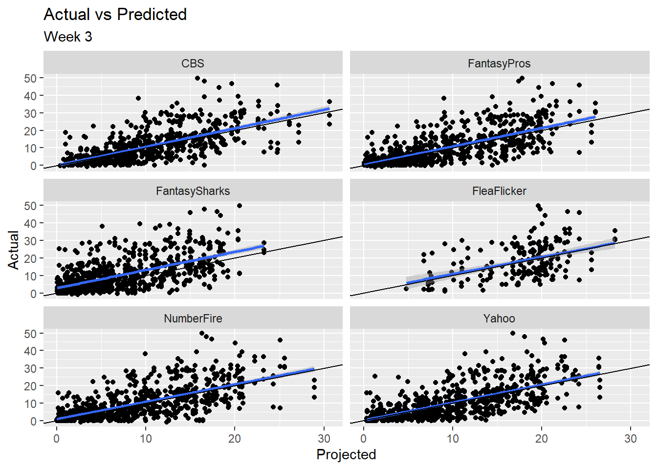
Tough to see much of a difference between sites here, with the exception of potentially a missing data issue with FleaFlicker. All fitted lines pretty closely hug the reference line, and the errors around those lines are fairly consistent. Now I’ll look at the distribution of errors by site to see if there’s anything we can identify.
comp %>%
  mutate(resid=dk_pts_actual-dk_pts_proj) %>%
  ggplot(aes(y=resid, x=data_src)) +
  geom_half_boxplot(side='r') +
  geom_half_violin(side='l', fill='darkblue') +
  ylab('Actual-Predicted') +
  xlab('Source') +
  ggtitle('Site Error Comparisons')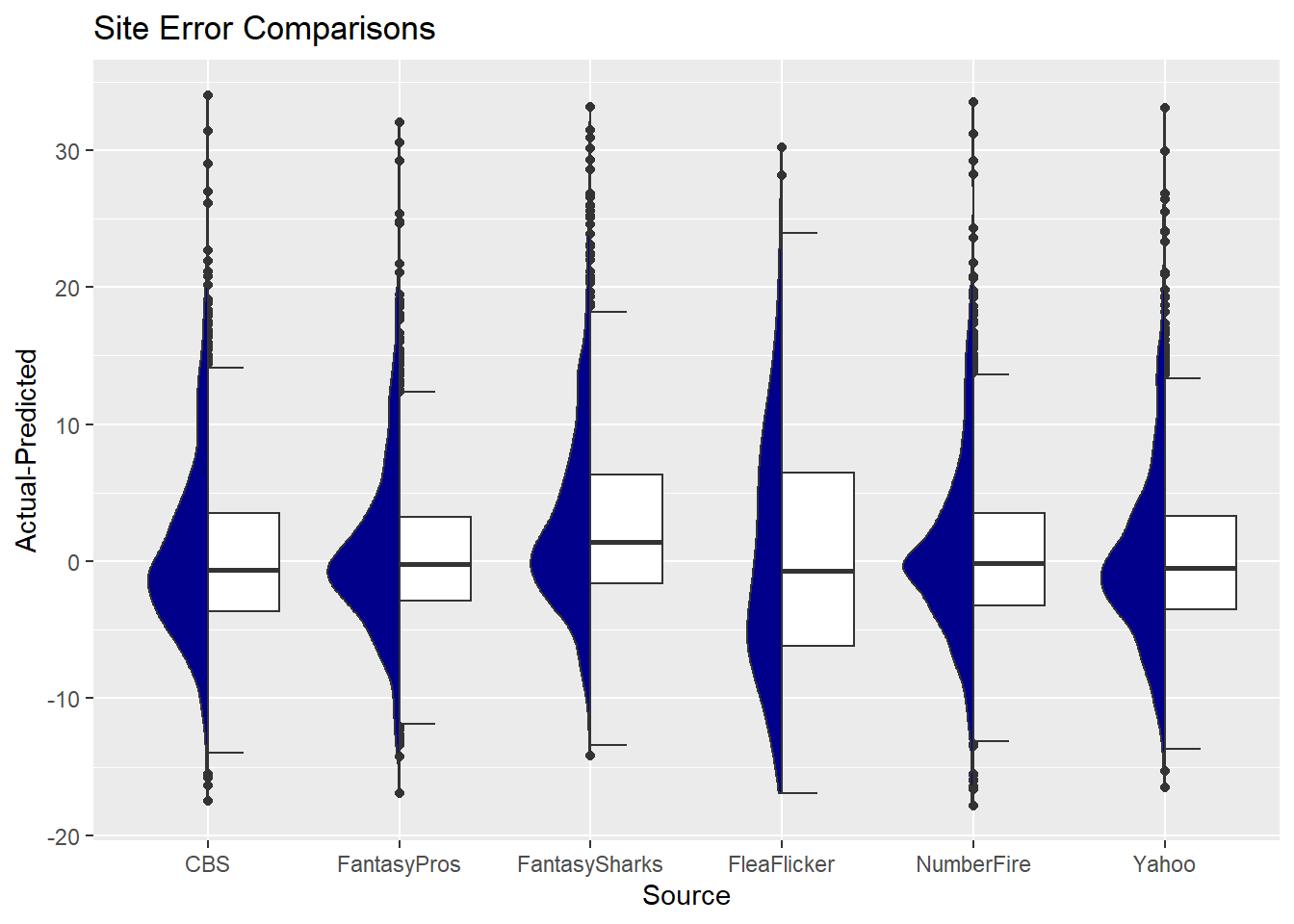
Here we get a bit of a better look of some differences. Looking closely, FantasyPros probably looks the best, followed by NumberFire. FleaFlicker (perhaps due to data issues) and FantasySharks look the worst here.
(Side Note: Did these with the new gghalves package I came across on twitter. Check it out here)
Conclusion
Now we have some idea of uncertainty levels around fantasy predictions, and there are some indicators of how each site is doing in comparison with the others. The question now is how these play out over the season, was FantasyPros just hot this week, or are they systematically more accurate than other sites? I hope to revisit this a few times throughout the season, so we can get answers!
